My First Solid Case: hotSphere
Case Overview
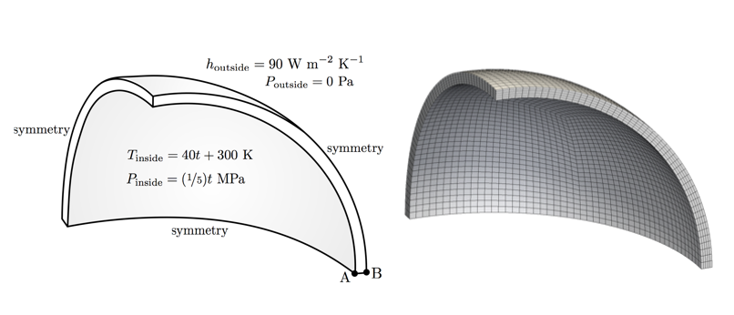
This case analyses the stresses and displacements generated in a spherical pressure vessel subjected to an increasing internal pressure and temperature.
The problem is 1-D axisymmetric in nature, but for demonstration purposes one eighth of the vessel is modelled here and symmetry planes are used.
The outer surface of the vessel is stress/traction free and the heat flux is given by Newton’s law of cooling (a simplified convection boundary condition).
*internal pressure and temperature are a function of time
Expected Results
Theory
-
We expect the vessel to deform due to the applied pressure and also due to the thermal gradient.
-
The deformations (strains/rotations) are expected to be “small”: this means we can use a small strain (linear geometry) approach, where the displacements are assumed not to affect the material geometry.
-
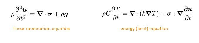
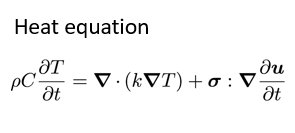
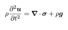
The conservation equations are linear momentum (linear geometry form) and energy (heat equation form):
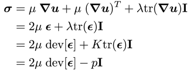
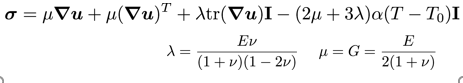
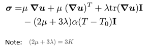
- Finally we will assume the deformation to be elastic (no permanent deformation) and the stress to be given by the Duhamel-Neumann form of Hooke’s law (i.e. Hooke’s law with thermal stress term):
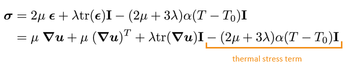
- Three mechanical properties must be specified: Elastic/Young’s modulus (E), Poisson’s ratio (ν) and the coefficient of linear thermal expansion (α). The Lamé parameters are then calculated as:
Theory: solution methodology
- This case employs a segregated solution methodology, where a loop is performed over the momentum equation (solved for displacement) and the energy equation (solved for temperature) until convergence is achieved. This loop is performed within each time-step resulting in an overall method that is implicit in time.
for all time-steps
    do
        solve energy equation for T (terms depending on D
        are calculated explicitly)

        solve momentum equation for D (terms depending on
        T are calculated explicitly)
    while not converged
end
Running the Case
The solids4foam tutorials are organised into fluids, solids and fluid-solid interaction cases, where the solid tutorials are further categorised by physical phenomena:
tutorials
├── …
├── fluidSolidInteraction
│   └── …
├── fluids
│   └── …
└── solids
    ├── elastoplasticity
    ├── fracture
    ├── hyperelasticity
    ├── linearElasticity
    ├── multiMaterial
    ├── poroelasticity
    ├── thermoelasticity
    └── viscoelasticity
Change directory to the “run” directory (create the directory if needed):
$> mkdir -p $FOAM_RUN && run
Copy the solids4foam tutorials to the run directory; note: it is assumed here that solids4foam is installed at “$FOAM_RUN/..”, like in the Docker image:
$> cp -r ../solids4foam/tutorials .
Change directory into the hotSphere tutorial case:
$> cd tutorials/solids/thermoelasticity/hotSphere
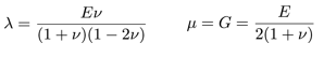
Run the case using the Allrun script and look at the results in ParaView:
$> ./Allrun
$> paraFoam   # or “paraFoam -nativeReader”
$> # or “touch case.foam && paraview case.foam”
If you are using the solids4foam docker image, it is not possible to directly open ParaView from within the image; so a workaround is to copy the tutorials to the shared directory in the docker container “/home/app/foam/app-4.0/sharedRun”: this directory points directly to the $HOME directory on your physical computer:
$> run
$> cd ../sharedRun
$> cp -r ../solids4foam/tutorials .
You can now open a second terminal (on your physical computer, NOT in the docker container) and use ParaView installed on your physical computer to view the cases in your $HOME directory.
Example of using ParaView on your physical computer to view cases created in the docker container:
- Docker terminal
$> mkdir -p $FOAM_RUN && run $> cd ../sharedRun $> cp -r ../solids4foam/tutorials . $> cd tutorials/solids/thermoelasticity/hotSphere $> ./Allrun - Followed by: Physical computer terminal
$> cd
$> cd tutorials/solids/thermoelasticity/hotSphere
$> touch case.foam && paraview case.foam
$> # or paraFoam
$> # or paraFoam -nativeReader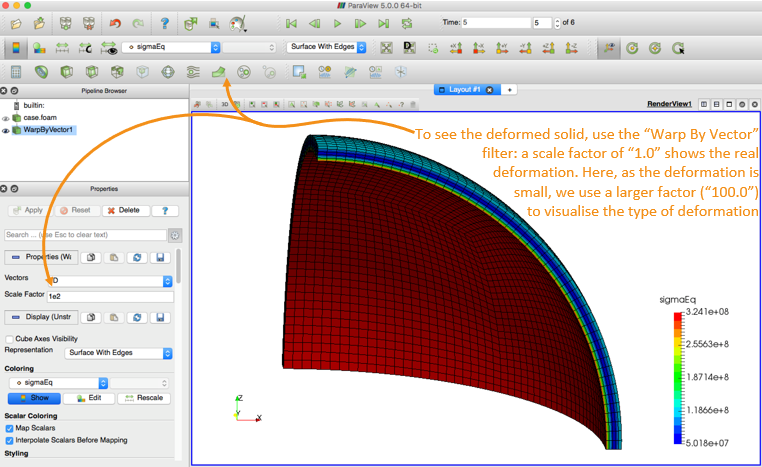
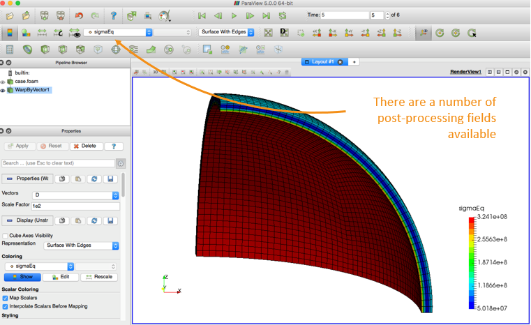
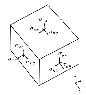
The stress tensor has 6 components
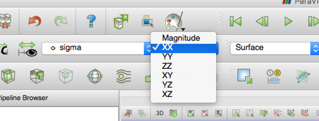
The von Mises stress (aka equivalent stress, sigmaEq) is commonly used to assess regions closest to failure:

The strain tensor also has 6 components; and we can define an equivalent strain compatible with the equivalent stress.
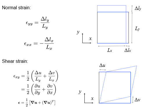
*These definitions of strain are only correct when the strains AND rotations are small; otherwise, see large/finite strain measures (e.g. Green strain, true strain) in e.g. Mase, Male, 1999, Continuum Mechanics for Engineers
Let us examine the hotSphere case structure in more detail …
hotSphere
├── 0
│   ├── D
│   └── T
├── Allclean
├── Allrun
├── constant
│   ├── dynamicMeshDict
│   ├── g
│   ├── mechanicalProperties
│   ├── physicsProperties
│   ├── polyMesh
│   │   └── …
│   ├── solidProperties
│   ├── thermalProperties
│   ├── timeVsPressure
│   └── timeVsTemperature
├── hotSphere.msh
└── system
    ├── controlDict
    ├── fvSchemes
    └── fvSolution
In this case, there are two primitive variables:
- displacement (vector)
- temperature (scalar)
├── 0
│   ├── D   displacement vector field
│   └── T   temperature scalar field
For displacement, we specify a zero-traction condition on the outer wall:
outside
{
  type            solidTraction;
  traction        uniform ( 0 0 0 );
  pressure        uniform 0;
  value           uniform (0 0 0);
}
Note: pressure here is referring to the normal component of the boundary traction vector: in general, this is not the same as the hydrostatic pressure. The total applied traction is: appliedTraction = traction - n*pressure where n is the boundary unit normal field and a time-varying traction condition on the inside wall:
inside
{
  type            solidTraction;
  traction        uniform ( 0 0 0 );
  pressureSeries
  {
      fileName “$FOAM_CASE/constant/timeVsPressure";
      outOfBounds clamp;
  }
  value           uniform (0 0 0);
}
where timeVsPressure specifies time vs pressure:
(
  ( 0 0 )
  ( 5 1e6 )
)
For the temperature field, we specify a convection condition (Newton’s law of cooling) on the outside:
outside
{
  type            thermalConvection;
  alpha           uniform 90;
  Tinf            300;
  value           uniform 300;
}
and a time-varying temperature on the inside wall:
inside
{
    type            fixedTemperature;
    temperatureSeries
    {
       fileName "$FOAM_CASE/constant/timeVsTemperature";
       outOfBounds clamp;
    }
    value           uniform 300;
}
where timeVsTemperature specifies time vs temperature:
(
    ( 0 300 )
    ( 5 500 )
)
Each tutorial contains an Allrun and Allclean script to run and clean/reset the case, e.g.
$> Allrun
Examining the Allrun script, this case requires two steps to run: create the mesh, and run the the solids4Foam solver:
$> fluentMeshToFoam hotSphere.msh
$> solids4Foam
Note: the mesh can be created in any external meshing software and then imported into OpenFOAM
All solids4foam cases require the physicsProperties dictionary; this allows the user to specify a fluid analysis, solid analysis, or fluid-solid interaction analysis:
│   ├── dynamicMeshDict
│   ├── g
│   ├── mechanicalProperties
│   ├── physicsProperties
│   ├── polyMesh
│   │   └── …
│   ├── solidProperties
│   ├── thermalProperties
│   ├── timeVsPressure
│   └── timeVsTemperature
├── hotSphere.msh
└── system
//type  fluid;
type    solid;
//type  fluidSolidInteraction;
In this case, we can see it is a solid analysis.
If a solid analysis is selected in the physicsProperties dictionary, then solids4Foam will look for the solidProperties dictionary in the constant directory.
Similarly, the fluidProperties dictionary is required for a fluid analysis, and the fsiProperties dictionary for a fluid-solid interaction analysis.
These dictionaries let us specify the details of what type of solid, fluid or fluid-solid interaction analysis is to be performed.
The solidProperties dictionary specifies:
solidModel
thermalLinearGeometry;

thermalLinearGeometryCoeffs
{
    nCorrectors          10000;

    solutionTolerance    1e-6;

    alternativeTolerance 1e-7;

    infoFrequency        100;
}
The thermalLinearGeometry is a solid mathematical model where the heat equation is solved (thermal-) and a linear geometry (-LinearGeometry) mechanical approach is taken.
A linear geometry approach is also known as a “small strain” or “small strain/rotation” approach and means that we assume the cell geometry (volumes, face areas, etc.) to be independent of the displacement field.
This assumption is typically OK when the deformation is “small”. Nonlinear geometry approaches (large strain approaches) are outside the scope of this training.
Remember the equations discussed previously in the “Theory” section; we will go through the relevant code later, and also the meaning of these settings.
A “solid” analysis requires the definition of the mechanical properties via the mechanicalProperties dictionary; in this case the thermoLinearElastic law is specified (Duhamel-Nuemann form of Hooke’s law):
mechanical
(
    steel
    {
        type  thermoLinearElastic;
        rho   rho [1 -3 0 0 0 0 0] 7750;
        E     E [1 -1 -2 0 0 0 0] 190e+9;
        nu    nu [0 0 0 0 0 0 0] 0.305;
        alpha alpha [0 0 0 -1 0 0 0] 9.7e-06;
        T0    T0 [0 0 0 1 0 0 0] 300;
    }
);
As we are performing a heat analysis, we also need to specify the thermal properties via the thermalProperties dictionary; in this case the constant law is specified (Fourier’s conduction law) by specific heat (C) and thermal conductivity (k):
thermal
{
    type      constant;
    C         C [0 2 -2 -1 0 0 0] 486;
    k         k [1 1 -3 -1 0 0 0] 20;
}
In all cases, we must also specify a dynamicMeshDict; in this case, it is set to staticFvMesh, which does not change the mesh during the simulation:
dynamicFvMesh staticFvMesh;
and the gravity field (g) must be specified: here we set it to zero to disable it. Try set it (0 -9.81 0) and see how it affects the results.
dimensions      [0 1 -2 0 0 0 0];
value           ( 0 0 0 );
hotSphere: running the solver
Let us now examine the output from the solids4Foam solver; first clean the case and prepare the mesh:
$> ./Allclean && fluentMeshToFoam hotSphere.msh
Next run the solids4Foam solver:
$> solids4Foam
We will look at the solver output …
Time = 1

Evolving thermal solid solver
Solving coupled energy and displacements equation for T and D
    Corr, res (T & D), relRes (T & D), matRes, iters (T & D)
    100, 3.37856e-10, 9.48897e-06, 0, 3.1907e-05, 0, 0, 12
    200, 1.97288e-10, 2.07022e-06, 0, 7.17093e-06, 0, 0, 10
    300, 9.26738e-10, 4.86841e-07, 0, 1.6726e-06, 0, 0, 10
    The residuals have converged
    337, 1.64639e-10, 2.83573e-07, 0, 9.86025e-07, 0, 0, 12

Max T = 340
Min T = 301.118
Max magnitude of heat flux = 321505
Max epsilonEq = 0.000254994
Max sigmaEq (von Mises stress) = 5.56883e+07
ExecutionTime = 8.73 s  ClockTime = 9 s
In general, the solver checks 3 types of residuals for the “solid”:
- res (linear solver residual)
- relRes (relative residual: change of the primitive variable)
- matRes (material residual: for nonlinear material laws)
where the tolerance is specified in the solidProperties dictionary. In this case, there are residuals for T and D; also, the material residual is zero because a linear mechanical law was selected (no need to iterate)
hotSphere: running the solver in parallel
To run the solids4Foam solver in parallel for solid and fluid cases (we will examine fluid-solid interaction later), copy the decomposeParDict into the case:
$> cp $FOAM_UTILITIES/parallelProcessing/decomposePar/decomposeParDict system/
Edit the decomposeParDict (e.g. using emacs - in the docker container, you can install emacs or vim using e.g. “apt-get install vim”) to use the “simple” method with 4 cores:
numberOfSubdomains  4;
method              simple;
simpleCoeffs
{
    n           (2 2 1);
    delta       0.001;
}
Then decompose the case (the cellist option creates a field for visualisation in ParaView showing the decomposition):
$> decomposePar -cellDist
Run the solver in parallel:
$> mpirun -np 4 solids4Foam -parallel
View the results in ParaView in parallel, or reconstruct the results first and view them in serial:
$> reconstructPar
$> paraFoam # or “paraFoam -nativeReader”
$> # or “touch case.foam && paraview case.foam”
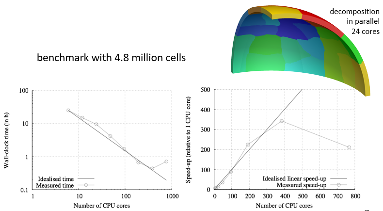
hotSphere: parallelisation
Case Settings
Next, we will explain the purpose of different numerical settings (physical properties, such as g, mechanicalProperties and thermalProperties are explained previously):
- solidProperties
- fvSchemes
- fvSolution
hotSphere
├── 0
│   ├── D
│   └── T
├── Allclean
├── Allrun
├── constant
│   ├── dynamicMeshDict
│   ├── g
│   ├── mechanicalProperties
│   ├── physicsProperties
│   ├── polyMesh
│   │   └── …
│   ├── solidProperties
│   ├── thermalProperties
│   ├── timeVsPressure
│   └── timeVsTemperature
├── hotSphere.msh
└── system
  ├── controlDict
  ├── fvSchemes
  └── fvSolution
Case numerical settings: solidProperties
As noted previously, the chosen solidModel is specified in the solidProperties dictionary; additionally, numerical settings and tolerances for the chosen solidModel can be specified (most be default to a good choice). Examining the hotSphere case, we see:
solidModel     thermalLinearGeometry;

thermalLinearGeometryCoeffs
{
    // Maximum number of correctors
    nCorrectors     10000;

    // Solution tolerance
    solutionTolerance 1e-6;

    // Alternative solution tolerance
    alternativeTolerance 1e-7;

    // Write frequency for the residuals
    infoFrequency  100;
}
- These four settings refer to the outer loop around the momentum (and heat) equation. Iterations will continue until either the D (and T) have converged to the specific tolerances, or the maximum number of correctors has been reached. If nCorrectors is reached, this means the equations have not converged to the required tolerance! The frequency of writing residuals to the standard output is controlled by infoFrequency.
Case numerical settings: fvSchemes
Switching between steadyState and transient analyses requires changing the d2dt2 and ddt schemes.
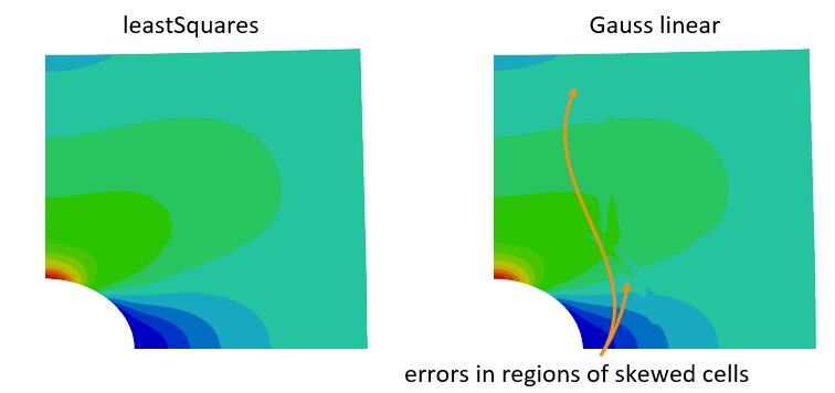
The gradient schemes should almost always be “leastSquares” as the standard “Gauss linear” method can produce large errors in the stress field for skewed cells.
d2dt2Schemes
{
    default            Euler; // or steadyState
}

ddtSchemes
{
    default            Euler; // or steadyState
}

gradSchemes
{
    default            leastSquares;
}

divSchemes
{
    default            Gauss linear;
}

laplacianSchemes
{
    default            Gauss linear corrected;
}

snGradSchemes
{
    default            corrected;
}

interpolationSchemes
{
    default            linear;
}
Case numerical settings: fvSolution
The D (and T) equations are very similar to the p equation in standard CFD approaches; as such, the conjugate gradient (PCG) or the algebraic multi-grid (GAMG) linear solvers tend to work best. The relTol can set be 0.1 as outer iterations are performed over the momentum equation until convergence.
In general, the D equation and field do not require under-relaxation; however, in some cases (e.g. in contact analysis) equation relaxation can help, or for poor meshes, field relaxation can help.
Relaxation factors less than 0.1 will be result in a prohibitively slow solution procedures.
solvers
{
    "D|DD|T"
    {
        solver          PCG;
        preconditioner  FDIC;
        tolerance       1e-09;
        relTol          0.1;
    }
}

relaxationFactors
{
    equations
    {
        //D    0.999;
    }
    fields
    {
        //D    0.7;
    }
}
Code
hotSphere: examining the code
The solids4foam toolbox structure is similar to that of OpenFOAM:
solids4foam
├── Allwclean
├── Allwmake
├── README.md
├── ThirdParty
├── applications
│   ├── solvers
│   │   └── solids4Foam
│   └── utilities
├── filesToReplaceInOF
├── src
│   ├── …
│   └── solids4FoamModels
└── tutorials
- Scripts to compile and clean the toolbox:
  $> ./Allwmake
  $> ./Allwclean
The README file briefly describes the toolbox.
solids4foam requires some ThirdParty code (e.g. Eigen header library): this is automatically downloaded (and compiled if needed) in the ThirdParty directory
-
The applications directory contains the solver and utilities: there is only one solver, it is called solids4Foam.
The utilities are for pre- and post-processing.
filesToReplaceInOF contains source code files from the main OpenFOAM libraries with bug-fixes: the Allwmake script will ask you to copy these into place.
-
The src directory contains the solids4FoamModels library (as well as others) used by the solids4Foam solver, including the fluid, solid and fluidSolidInteraction algorithms.
As discussed previously, the tutorial directory contains example cases for fluid, solid and fluidSolidInteraction analyses.
Let us examine the solids4Foam solver code:
solids4foam/applications/solvers/solids4Foam/solids4Foam.C
int main(int argc, char *argv[])
{
#   include "setRootCase.H"
#   include "createTime.H"
#   include "solids4FoamWriteHeader.H"

    // Create the general physics class
    // This is a run-time selectable class, so within the case we can decide to
    // solve a fluid, solid or fluid-solid interaction model
    autoPtr<physicsModel> physics = physicsModel::New(runTime);
    while (runTime.run())
        {
            // Update deltaT, if desired, before moving to the next step
            // Fluid or solid methodologies may have time-step limitations

            physics().setDeltaT(runTime);

            runTime++;

            Info<< "Time = " << runTime.timeName() << nl << endl;

            // This is where the mathematical model equations will be solved, e.g.
            // fluid equations, solid equations, or both for fluid-solid interaction

            physics().evolve();

            // This function lets the physics model know we have reached the end of
            // of the time-step, in case it needs to update fields

            physics().updateTotalFields();
            if (runTime.outputTime())
        {
            // Solid physics models often create and write extra fields when
            // fields are being written
            physics().writeFields(runTime);
        }

        Info<< "ExecutionTime = " << runTime.elapsedCpuTime() << " s"
            << "  ClockTime = " << runTime.elapsedClockTime() << " s"
            << nl << endl;
    } // end of time loop

    // Let the physics model know it is the end of the simulation in case it needs
    // to clean anything up
    physics().end();

    Info<< nl << "End" << nl << endl;

    return(0);
}
Physics Model
The physicsModel is an abstract base class, where there are currently three derived classes:
- fluidModel
- solidModel
- fluidSolidInterface, where fluidSolidInterface creates its own fluidModel and solidModel
Each of these three classes are also abstract base classes, where specific fluid, solid, and fluid-solid interaction implementations derive from them: see next slide.
hotSphere: examining the code
Examining the solids4FoamModels library structure: solids4foam
├── ...
└── src
    ├── …
    └── solids4FoamModels
        ├── ...
        ├── dynamicFvMesh
        ├── fluidModels
        ├── fluidSolidInterfaces
        ├── functionObjects
        ├── materialModels
        ├── numerics
        ├── physicsModel
        └── solidModels
The fluidModels, solidsModels and fluidSolidInterfaces are stored in separate directories.
In addition, the physicsModel is located here.
Physics Model: Fluid Models
For example, there are currently a number of fluid models implementations that derive from the fluidModel base class:
- icoFluid
- pUCoupledFluid
- pisoFluid
- transientSimpleFluid
- interFluid
- buoyantBoussinesqPimpleFluid
- …
Each of these fluidModels corresponds to a standard fluid solver in OpenFOAM, which has been repackaged into a class form.
Physics Model: Solis Models
The solid models implementations, deriving from the solidModel base class, include:
- linGeomSolid
- thermalLinGeomSolid
- coupledUnsLinGeomLinearElasticSolid
- nonLinGeomTotalLagSolid
- nonLinGeomUpdatedLagSolid
- poroLinGeomSolid
- …
Physics Model: Fluid-Solid Interaction Models
The fluid-solid interaction models implementations, deriving from the fluidSolidInterface base class, include:
- fixedRelaxationCouplingInterface
- AitkenCouplingInterface
- IQNILSCouplingInterface
- weakCouplingInterface
- oneWayCouplingInterface
- …
Each method employs a different approach for coupling the fluid and the solid domains.
hotSpere: code
For the hotSphere test case, we have selected a “solid” analysis in the physicsProperties dictionary: this means a solidModel class will be selected; then, we specify the actual solidModel class to be the thermoLinGeomSolidModel class.
The code for the thermoLinGeomSolidModel class is located at:
solids4foam/src/solids4FoamModels/solidModels/thermalLinGeomSolid/thermalLinGeomSolid.C
Let us examine the “evolve” function of this class to see the equations solved…
bool thermalLinGeomSolid::evolve()
{
    Info<< "Evolving thermal solid solver" << endl;

    int iCorr = 0;
    lduSolverPerformance solverPerfD;
    lduSolverPerformance solverPerfT;
    blockLduMatrix::debug = 0;

    Info<< "Solving coupled energy and displacements equation for T and D"
        << endl;

    // Momentum-energy coupling outer loop
    do
    {
        // Store fields for under-relaxation and residual calculation
        T().storePrevIter();

        // Heat equation
        fvScalarMatrix TEqn
        (
            rhoC_*fvm::ddt(T_)
         == fvm::laplacian(k_, T_, "laplacian(k,T)")
          + (sigma() && fvc::grad(U()))
        );
...
- Note: U in the code is velocity and D is displacement; however, in the slides u represents displacement
        // Under-relaxation the linear system
        TEqn.relax();

        // Solve the linear system
        solverPerfT = TEqn.solve();

        // Under-relax the field
        T_.relax();

        // Update gradient of temperature
        gradT_ = fvc::grad(T_);

        // Store fields for under-relaxation and residual calculation
        D().storePrevIter();

        // Linear momentum equation total displacement form
        fvVectorMatrix DEqn
        (
            rho()*fvm::d2dt2(D())
         == fvm::laplacian(impKf_, D(), "laplacian(DD,D)")
          - fvc::laplacian(impKf_, D(), "laplacian(DD,D)")
          + fvc::div(sigma(), "div(sigma)")
          + rho()*g()
          + mechanical().RhieChowCorrection(D(), gradD())
        );
...
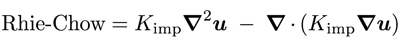
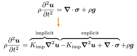
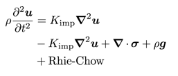
- Also, we add an additional diffusion term to quell numerical oscillations (e.g. checker-boarding) based on Rhie-Chow correction:
        // Under-relaxation the linear system
        TEqn.relax();

        // Solve the linear system
        solverPerfT = TEqn.solve();

        // Under-relax the field
        T_.relax();

        // Update gradient of temperature
        gradT_ = fvc::grad(T_);

        // Store fields for under-relaxation and residual calculation
        D().storePrevIter();

        // Linear momentum equation total displacement form
        fvVectorMatrix DEqn
        (
            rho()*fvm::d2dt2(D())
         == fvm::laplacian(impKf_, D(), "laplacian(DD,D)")
          - fvc::laplacian(impKf_, D(), "laplacian(DD,D)")
          + fvc::div(sigma(), "div(sigma)")
          + rho()*g()
          + mechanical().RhieChowCorrection(D(), gradD())
        );
...
        // Under-relaxation the linear system
        DEqn.relax();

        // Solve the linear system
        solverPerfD = DEqn.solve();

        // Under-relax the field
        relaxField(D(), iCorr);

        // Update increment of displacement
        DD() = D() - D().oldTime();

        // Update velocity
        U() = fvc::ddt(D());

        // Update gradient of displacement
        mechanical().grad(D(), gradD());

        // Update gradient of displacement increment
        gradDD() = gradD() - gradD().oldTime();

        // Calculate the stress using run-time selectable mechanical law
        mechanical().correct(sigma());
...
- Stress is calculated by run-time selectable mechanicalLaw, chosen in the mechanicalProperties dictionary
// Update impKf to improve convergence // Note: impK and rImpK are not updated as they are used for traction // boundaries if (iCorr % 10 == 0) { impKf_ = mechanical().impKf(); } } while ( !converged(iCorr, solverPerfD, solverPerfT, D(), T_) && ++iCorr < nCorr() ); // loop around TEqn and DEqn // Interpolate cell displacements to vertices mechanical().interpolate(D(), pointD()); // Increment of displacement DD() = D() - D().oldTime(); // Increment of point displacement pointDD() = pointD() - pointD().oldTime(); return true; } - Choice of impK can affect convergence (but not the answer - assuming convergence is achieved) i.e. tangent matrix in finite element analysis
MechanicalLaw: code
For the hotSphere test case, we have selected the thermoLinearElastic mechanical law in the case mechanicalProperties dictionary: this class will perform the calculation of stress for the solid.
The code for the thermoLinearElastic mechanical law class is located at:
solids4foam/src/solids4FoamModels/materialModels/mechanicalModel/mechanicalLaws/linearGeometryLaws/thermoLinearElastic/thermoLinearElastic.C
Let us examine the “correct” function of this class to see how the stress is calculated …
Duhamel-Neumann form of Hooke’s law:
void Foam::thermoLinearElastic::correct(volSymmTensorField& sigma)
{
    // Calculate linear elastic stress
    linearElastic::correct(sigma);

    if (TPtr_.valid())
    {
        // Add thermal stress component
        sigma -= 3.0*K()*alpha_*(TPtr_() - T0_)*symmTensor(I);
    }
    else
    {
        // Lookup the temperature field from the solver
        const volScalarField& T = mesh().lookupObject<volScalarField>("T");

        // Add thermal stress component
        sigma -= 3.0*K()*alpha_*(T - T0_)*symmTensor(I);
    }
}
As thermoLinearElastic derives from the linearElastic law, we will also examine the “correct” function for this class:
solids4foam/src/solids4FoamModels/materialModels/mechanicalModel/mechanicalLaws/linearGeometryLaws/linearElastic/linearElastic.C ``` void Foam::linearElastic::correct(volSymmTensorField& sigma) { // Calculate total strain if (incremental()) { // Lookup gradient of displacement increment const volTensorField& gradDD = mesh().lookupObject
("grad(DD)");
    epsilon_ = epsilon_.oldTime() + symm(gradDD);
}
else
{
    // Lookup gradient of displacement
    const volTensorField& gradD =
        mesh().lookupObject<volTensorField>("grad(D)");

    epsilon_ = symm(gradD);
}
// For planeStress, correct strain in the out of plane direction
    if (planeStress())
    {
        if (mesh().solutionD()[vector::Z] > -1)
        {
            FatalErrorIn
            (
                "void Foam::linearElasticMisesPlastic::"
                "correct(volSymmTensorField& sigma)"
            )   << "For planeStress, this material law assumes the empty "
                << "direction is the Z direction!" << abort(FatalError);
        }

        epsilon_.replace
        (
            symmTensor::ZZ,
        -(nu_/E_)
        *(sigma.component(symmTensor::XX) + sigma.component(symmTensor::YY))
        );
    }
    // Hooke's law : standard form
//sigma = 2.0*mu_*epsilon_ + lambda_*tr(epsilon_)*I + sigma0_;

// Hooke's law : partitioned deviatoric and dilation form
const volScalarField trEpsilon = tr(epsilon_);
calculateHydrostaticStress(sigmaHyd_, trEpsilon);
sigma = 2.0*mu_*dev(epsilon_) + sigmaHyd_*I + sigma0_; } ``` Standard Hooke’s law can be expressed in a number of equivalent forms: